This model stems from Kohonen (1982) and builds upon earlier work of Willshaw and von der Malsburg (1976). The model is similar to the (much later developed) neural gas model (see 5.1) since a decaying neighborhood range and adaptation strength are used. An important difference, however, is the topology which is constrained to be a two-dimensional grid (
The distance on this grid is used to determine how strongly a unit ![]() is adapted when the unit
is adapted when the unit ![]() is the winner.
The distance measure is the
is the winner.
The distance measure is the ![]() -norm (a.k.a. ``Manhattan distance''):
-norm (a.k.a. ``Manhattan distance''):
![]()
Ritter et al. (1991) propose to use the following function to
define the relative strength of adaptation for an arbitrary unit r in the
network (given that s is the winner):
![]()
Thereby, the standard deviation ![]() of the Gaussian is varied according
to
of the Gaussian is varied according
to
![]()
for a suitable initial value ![]() and a final value
and a final value ![]() .
The complete self-organizing feature map algorithm is the following:
.
The complete self-organizing feature map algorithm is the following:
Initialize the connection set ![]() to form a rectangular
to form a rectangular ![]() grid.
grid.
Initialize the time parameter t:
![]()
![]()
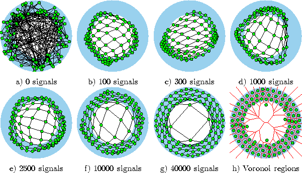
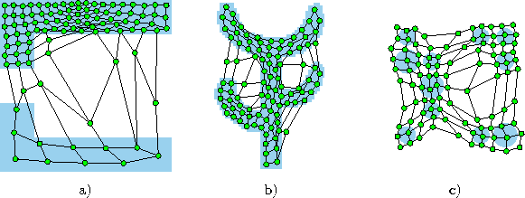
Figure 6.1 shows some stages of a simulation for a simple ring-shaped data distribution. Figure 6.2 displays the final results after 40000 adaptation steps for three other distribution.
The parameters were ![]() and
and ![]() .
.

Figure 6.1: Self-organizing feature map simulation sequence for a ring-shaped uniform probability distribution. a) Initial state. b-f) Intermediate states. g) Final state. h) Voronoi tessellation corresponding to the final state. Large adaptation rates in the beginning as well as a large neighborhood range cause strong initial adaptations which decrease towards the end.

Figure: Self-organizing feature map simulation results after 40000 input signals for three different probability distributions (described in the caption of figure 4.4).