

Next: Competitive Hebbian Learning
Up: Soft Competitive Learning without
Previous: Soft Competitive Learning without
The neural gas algorithm (Martinetz and Schulten, 1991) sorts for each input signal
 the units of the network according to the distance of their
reference vectors to
  . Based on this ``rank order'' a certain number of units
is adapted. Both the number of adapted units and the adaptation strength are decreased
according to a fixed schedule. The complete neural gas algorithm is the following:
- 1.
- Initialize the set
 to contain N units

with reference vectors  chosen randomly according to
 .
.
Initialize the time parameter t:

- 2.
- Generate at random an input signal
 according to
  .
.
- 3.
- Order all elements of
 according to their distance to
  ,
i.e., find the sequence of indices
  such that
 is the reference vector closest to
  ,
,  is the
reference vector second-closest to
  and
and  is the reference vector such that k vectors
  exist with
 . Following Martinetz et al. (1993) we denote
with
 the number k associated with
  .
.
- 4.
- Adapt the reference vectors according to

with the following time-dependencies:


- 5.
- Increase the time parameter t:

- 6.
- If
 continue with step 2
For the time-dependent parameters suitable initial values
 and final values
  have
to be chosen.
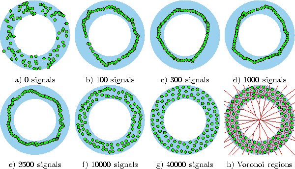
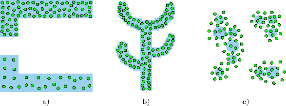
Figure 5.1 shows some stages of a simulation for a simple ring-shaped data distribution. Figure 5.2 displays the final results after 40000 adaptation steps for three other distribution.
Following
Martinetz et al. (1993) we used the following parameters:
 .
.

Figure 5.1: Neural gas simulation sequence for a ring-shaped uniform probability distribution. a) Initial state. b-f) Intermediate states. g) Final state. h) Voronoi tessellation corresponding to the final state. Initially strong neighborhood interaction leads to a clustering of the reference vectors which then relaxes until at the end a rather even distribution of reference vectors is found.

Figure: Neural gas simulation results after 40000 input signals for three different probability distributions (described in the caption of figure 4.4).


Next: Competitive Hebbian Learning
Up: Soft Competitive Learning without
Previous: Soft Competitive Learning without
Bernd Fritzke
Sat Apr 5 18:17:58 MET DST 1997
![]()
![]() and final values
and final values ![]() have
to be chosen.
Figure 5.1 shows some stages of a simulation for a simple ring-shaped data distribution. Figure 5.2 displays the final results after 40000 adaptation steps for three other distribution.
Following
Martinetz et al. (1993) we used the following parameters:
have
to be chosen.
Figure 5.1 shows some stages of a simulation for a simple ring-shaped data distribution. Figure 5.2 displays the final results after 40000 adaptation steps for three other distribution.
Following
Martinetz et al. (1993) we used the following parameters:
![]() .
.

